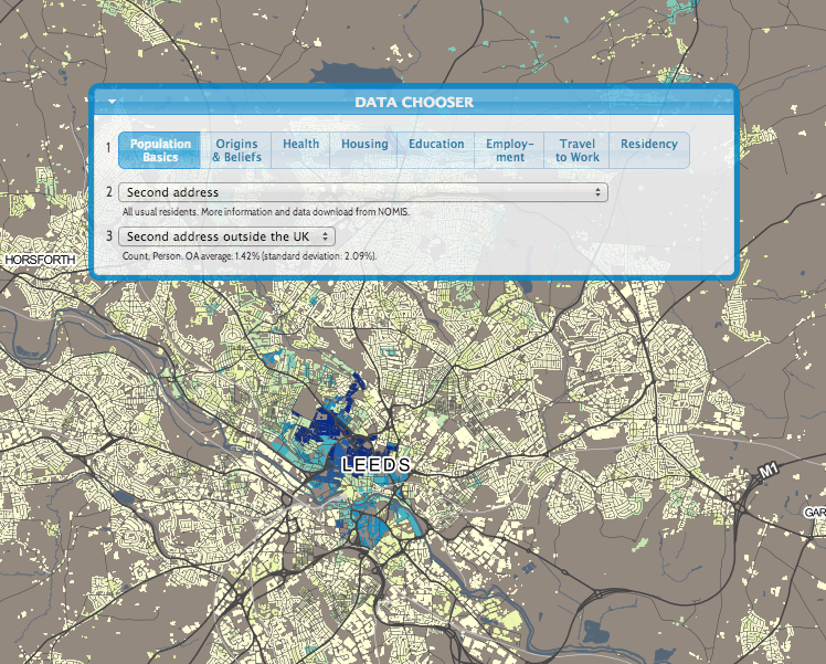
DataShine: Census is the first product of BODMAS’s DataShine toolkit. We have taken the Quick Statistics aggregate tables, released for the 2011 Census by the Office of National Statistics. We are using two geographies for these – Output Areas, which have a typical population of around 150-200 people, and Wards, which, being a political rather than statistical unit, vary more in population but typically have around 7000 in each. Wards have the advantage of having real names rather than numbers, and are manually designed to surround contiguous communities. As you zoom in and out of the DataShine Census maps, you’ll see the geographies change – Wards are simpler (so faster to create the maps) and because of their larger populations, have less of a patchwork look, particularly for datasets that have a very low average value or high variation.
The DataShine Census maps are generally maps showing the variation in percentages of a general population that fall into the selected category type. We have removed a small number of different maps in the dataset – such as population density – although hope to have these included in due course. We have also not, at this stage, included the Scottish and Northern Irish datasets, as these come as separate files. Again, we hope to have these in DataShine Census in time.
We decide how to map each data table based on the average percentage (for the current geography) and the standard deviation of the percentage values. Many census variables have very small average values (less than 1%) and standard deviations of the percentage and so are mapped as multiples of the average, or location quotient (LQ). For example, an LQ of 6 indicates the local area has six times the proportion of people (or households) in the selected category, than the England/Wales average for that geography. Other strategies are tried for different kinds of data.

great!