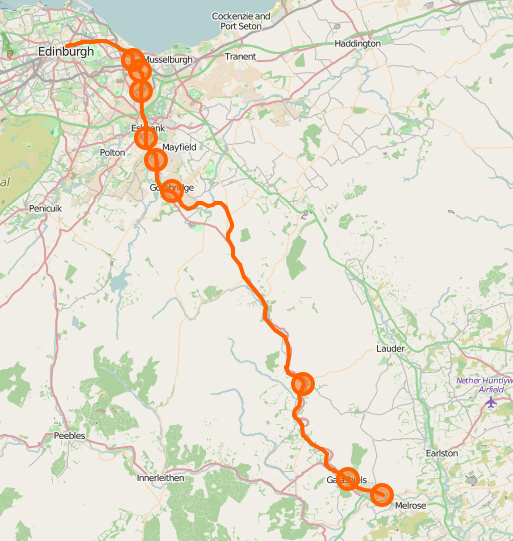
The Borders Railway opened last week – a 30 mile new railway running between Edinburgh and the Scottish Borders, which was for the last fifty years the largest populated region in the UK without a railway connection. The railway largely follows the route of the Waverley Line, which used to connect Edinburgh to Carlisle via the Borders (Galashiels and Hawick) before it was axed in the 1960s. The new line is highlighted in the map above, as are the small stations that lead to central Edinburgh at the end of the route. Galashiels is the penultimate station, with Tweedbank, a suburb of Galashiels, being the terminus.
This post looks at the pre-opening (i.e. Census 2011) commuting patterns between the western Borders towns, both those now connected to the new railway and those nearby but not linked, and Edinburgh. It’s a commute pattern that is personally interesting to me as I have childhood memories of waiting various “Munros” buses to come over the hills from the Borders, to get into Edinburgh. It also looks at the relative deprivation scores and potentially related census characteristics, between the towns.
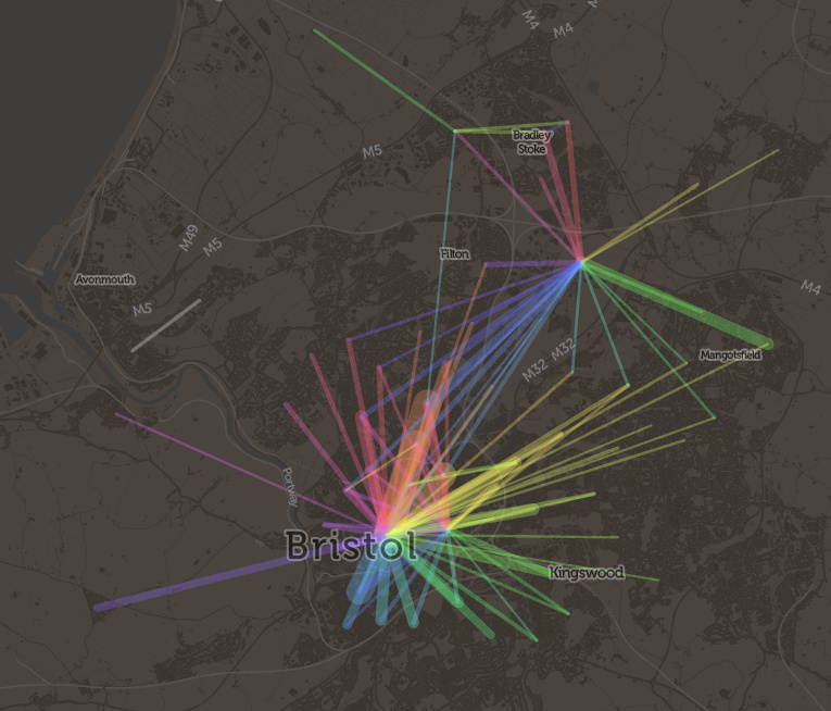
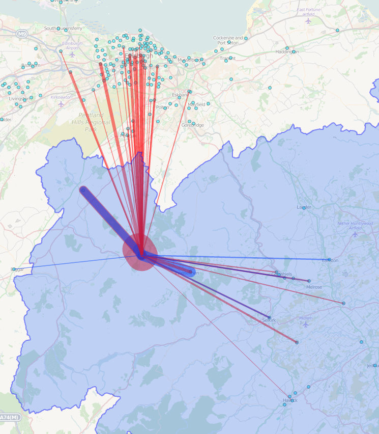
The graphics here are from our newly launched DataShine Scotland Commute which shows travel-to-work flows as straight-line origin/destination maps – it should be noted they don’t include any transnational commutes, e.g. from the Borders towns into Carlisle in England. For that, you need the DataShine Region Commute. The Borders council area is shaded in blue.
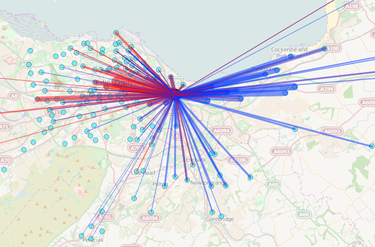
Here are four maps from towns (and surrounding areas), in the Borders region, near each other and approximately equidistant to Edinburgh, showing the flows out to work from people living in those areas (red) and flows in to work there from people living outside (blue). The four places I’m showing are, from west to east, Peebles, Innerleithen, Galashiels and Earlston.
Peebles:
Innerleithen:
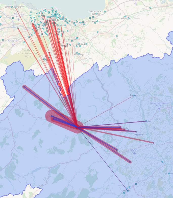
Galashiels North:
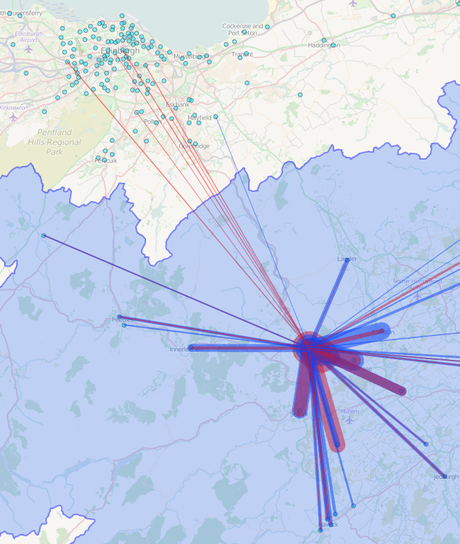
Earlston & surrounding area:
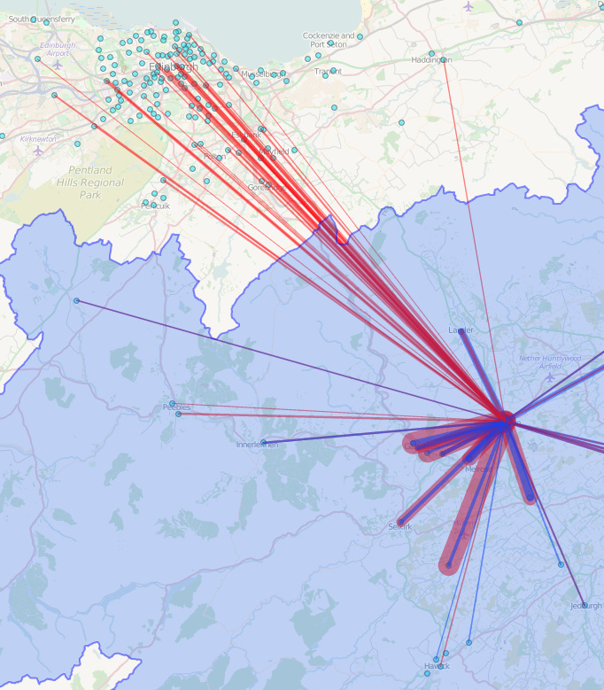
Notice the odd one out?
Galashiels, the one of the four to which the new Borders Railway now connects Edinburgh to shows a significantly smaller level of commuting activity (as of the 2011 Census) to Edinburgh, than the other three areas, all statistical areas having approximately equal populations, and which are approximately the same distance from Edinburgh (an 45-minute drive or an hour-long bus journey). You can see an interactive version for all four, and indeed anywhere else in Scotland, here. Instead, it shows most commuting activity remaining within the Border valleys. It has a much weaker social connection to Scotland’s capital city.
N.B. In Earlston’s case, the small population in the town means that local rural communities are also included in its data point. Conversely, Galashiels’ large population is split into three, I’ve chosen the northern one which is a little closer to Edinburgh and also likely includes Stow, a small village to the north and the next stop on the new Borders Railway. The other Galashiels areas are broadly similar in terms of their commuting patterns.
Looking at DataShine Scotland which looks instead at the “static” aggregated small-area Census data rather than the flows above, we can begin to understand more about the demographics of each of the four towns and why Galashiels Edinburgh links are weaker. Galashiels’ population is generally younger and less likely to be married. People of Galashiels are also less likely to declare themselves of being of “very good health” than the other three areas. A younger, less healthy population is potentially indicative of a more deprived area, this is confirmed via mapping the Scottish Index of Multiple Deprivation (SIMD) 2011. Galashiels has both more and less deprived areas (red and green), but stands out against Peebles, Innerleithen and Earlston, who are generally green/yellow and so do not have a significant deprived area.
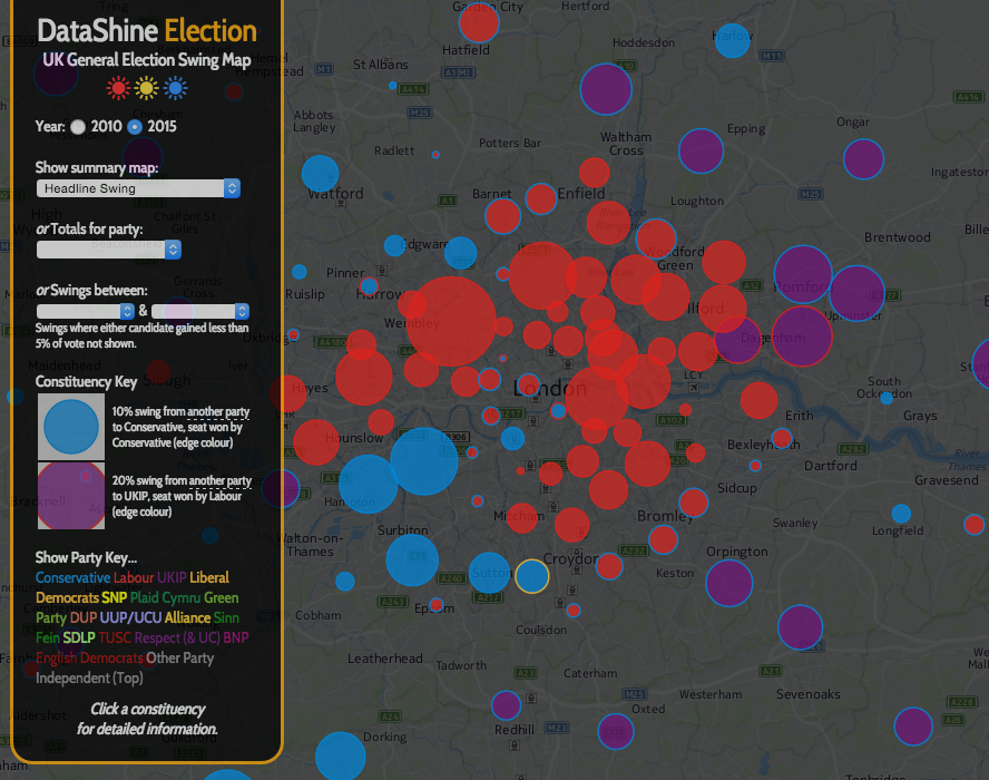
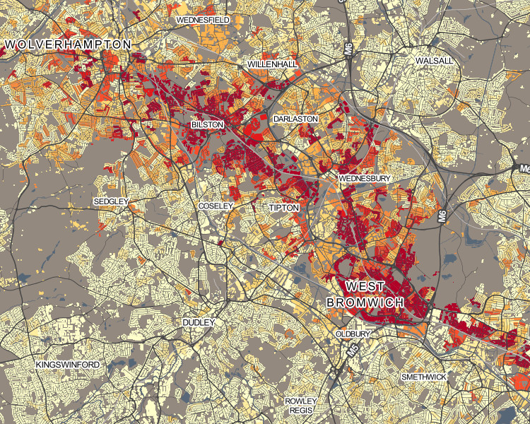
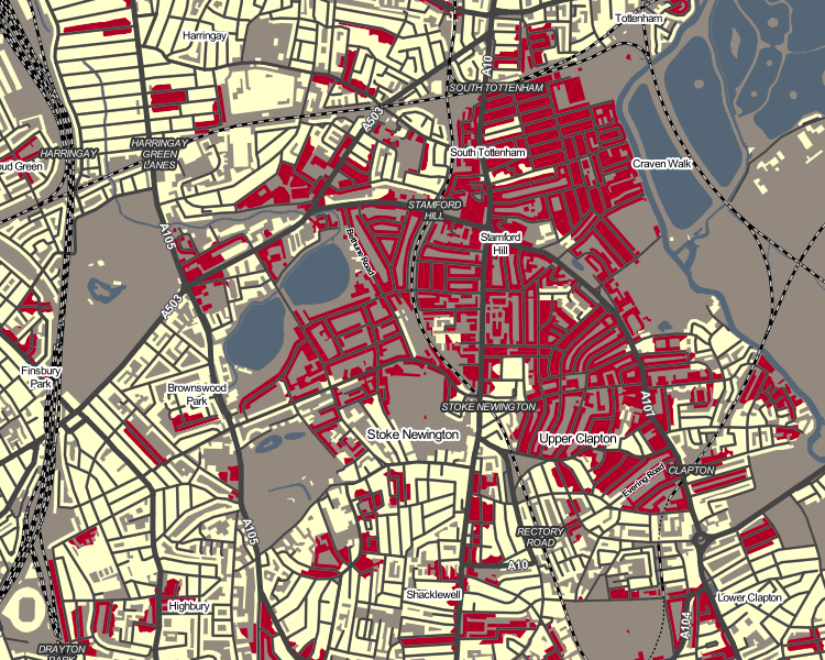
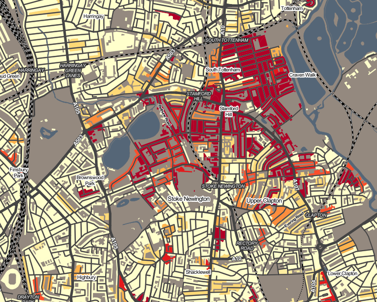
So perhaps poorer Galashiels, having little existing interaction with affluent Edinburgh, stands more to gain from the new, regular and fast connection to Scotland’s capital city, and that the new connection will, if it is used well, likely have a significant social impact on Galashiels and its fortunes, more so than would be gained from improving the other Borders towns. Renewed railway lines, as a method to transform the wealth of areas, is likely demonstrated by the dramatic effect on fortunes and house prices along the East London line in north-east London, following the reinstatement of the railway line there, and perhaps Galashiels and the surrounding areas will also see a step-change in the years to come?
Map data Copyright OpenStreetMap contributors 2015. Census data from NRS, Crown Copyright and database right 2015.